Managing inventory variability is a constant struggle in business one tool to help manage this is a regression analysis. A regression analysis is a statistical assessment of date that seeks to identify a general overlaying trend. It defines a sample set of date as a line. Like all statistical tools a regression analysis has limitations and without an intuition of the sample data a regression analysis is useless. The following is a sample of how a regression analysis could be used in small business inventory management and how knowledge of the real world implications was taken into account.
As an operations engineer of an aluminum and bronze casting facility that produces a proprietary line of electrical transmission components it was my job to address product requisitions, generate quotes and do what I can to make the fulfillment of orders go smoothly. One of the dilemmas that we faced was providing parts with a minimal lead time.
More often then not customers came to us looking for parts they needed quickly, and in the world of power transmission a day can mean thousands upon thousands of dollars lost. We did what we could to get the needed parts out as fast as we could but if a part was not on the shelf there would most certainly be a delay. It isn’t practical to maintain a large inventory all the time due to the carrying costs involved so, as an alternative we kept a select inventory of our most popular parts available.
As our name grew and more people heard about the product line, our market share also saw growth. This selective inventory model worked nicely for us but with the continual rise in sales comes a need for more parts on hand. The question became; at what rate should we continue to add to our selective inventory?
Each part had a separate demand so for the sake of this exercise I focused on only one item. I have gathered the quantities sold of this part over a 34 month period. The data is as follows:
|
Monthly |
|
|
date By Month |
Sum Of qty |
|
|
|
| January 2003 |
245 |
| February 2003 |
186 |
| March 2003 |
55 |
| April 2003 |
326 |
| May 2003 |
510 |
| June 2003 |
329 |
| July 2003 |
110 |
| August 2003 |
52 |
| September 2003 |
677 |
| October 2003 |
100 |
| November 2003 |
37 |
| December 2003 |
362 |
| January 2004 |
1014 |
| February 2004 |
45 |
| March 2004 |
136 |
| April 2004 |
186 |
| May 2004 |
196 |
| June 2004 |
60 |
| July 2004 |
213 |
| August 2004 |
239 |
| September 2004 |
191 |
| October 2004 |
151 |
| November 2004 |
32 |
| December 2004 |
190 |
| January 2005 |
1003 |
| February 2005 |
100 |
| March 2005 |
361 |
| April 2005 |
154 |
| May 2005 |
161 |
| June 2005 |
561 |
| July 2005 |
338 |
| August 2005 |
135 |
| September 2005 |
820 |
| October 2005 |
1259 |
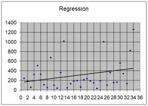
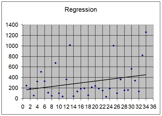
Now that we have the data we can plot a regression and see our trend. Using Excel QM we find the definition of this trend line to be Y=8.52X+160
As you can see our quantities are all over the place but there is an indication that we were experiencing an upward trend in our average volume.
This regression suggests that we were selling 8.52 additional parts every month. If this were the case it would be wise to add 8.52 additional parts to our on hand inventory every month to compensate. The result would be an out put that doubles roughly every 2 years.
A product that doubles in sales every two years is a great for a company but lets look at the over all sales for each year to see how they match up. Taking a step back to make sure we see the full picture proved to be prudent.
|
Yearly |
|
|
date By Year |
Sum Of qty |
|
|
|
| 2003 |
2989 |
| 2004 |
2653 |
| 2005 |
4892 |
The data that we used to generate our regression shows a dip in sales in 2004 and a spike in 2005. It would be wise to take note of this as the deviation in sales is a good indication that the demand is not constant. If our demand isn’t constant we need to be careful about producing more parts then what we can sell.
One way to combat this is to make the on site inventory a function of the prior month’s sales. Knowing that the ratio of standard orders to rush orders was about 7:1 we could determine a good starting point for our inventory to be 20% of the prior month’s sales. While this may result in a larger on site inventory then what is required for rush orders, it is more then likely not going to exceed the quantity that we will sell for the month.
Every bit of data helps us determine what tomorrow might bring but no extent of data will ever insure us as to what tomorrow will bring. The regression analysis provided an indication to our macro rate of change while a quick look at our over all sales showed us that the distribution of sales was not uniform.
A good practice would be to continually run the regression analysis for different time periods and see if perhaps we could identify potential cycles or seasonal trends that we could later exploit in order to maximize profit.
I hope this illustrates how a tool like a regression analysis can be helpful but could lead to making wrong decisions if the practical circumstances are not understood. Many people right out of college have a great deal of tools under their belt but often do not know how to properly us them in the real world. My hope is that this illustration will push you to better understand your problems before spouting off a potential solution.


Leave a Reply